COMMANDS WHICH CAN BE USED TO SOLVE THE TASKS

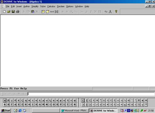
1.) We write an expression in the dialog box on the lower part. For example, if we want to do something with the logarithmic function with the base 10, we write log(x, 10) and conclude the input by pressing the “Enter” – key.

2.) Now we will plot the graph of the logarithmic function. We use the command Insert in the menu bar. This menu offers 4 commands. We use 2D – plot Object. Derive creates a plot window. We can sketch the curve, if we repeat command Insert and then use command Plot.

The other way to sketch the graph of the function is to click on the toolbar button twice.

3.) If you want to delete the curve, you choose the command Edit in the menu bar and one of the Delete commands in this menu.

4.) In order to switch between a plot and algebra window we have to choose the command Window and then choose one of the windows given below. Or we use the toolbar button to switch from the graphics window to the algebra window.

5.) Sometimes we have to change the unit size on co-ordinate axes. We use Set in the menu bar and the third choice Plot Region. We choose, for example, horizontal length 30 and 30 intervals, too. We don´t change the vertical length. With click on the OK key we get the co-ordinate axes with the new unit size.

6.) The family of functions, for example, is drawn by entering an expression , where is at the first place the function, at the second is the index variable and then the first value of the index variable and the last value of the index variable. At the end we can write the step size of the index variable. The default is a step size of 1. Then we simplify the expression by the command Simplify in the menu bar and with the offer Basic in this menu. We plot these as before.

7.) To write a title or annotation next to a picture we click the point where the annotation should start. By choosing Insert and Annotation we get the dialog box, which allows us to enter the annotation text.

We delete the annotation text, if we move the graphics cursor on the annotation text and choose Edit, Delete Annotation.

8.) Replacing an expression´s variable by specific value is called substitution. To substitute 3 for x in expression we perform the following steps: Simplify, Variable Substitution, we choose the new value 3 and click on the OK key. Then we approximate the expression with the command Simplify, Approximate, we choose digits of precision and choose Approximate once more. Of course, we can use the tool bar instead of the menu bar, too. The toolbar button for the approximate is . It is also possible to write the expression log(3, 10) and use only the last part of this instruction.

9.) We can solve the equation, for example or only on two different ways. The first is the exact way using the commands Solve, Expression, Algebraically, Solve. If we want to try to solve the first equation, Derive returns the equation in different form but still unsolved. This indicates that Derive cannot solve this problem. For the elementary equation the exact way is convenient. Therefore, the best way is an approximative solution with the order Solve, Expression, Numerically, Solve, which really gives us a solution.